To meet the challenges of scaling systems in size, scope, and complexity, it is useful to look at new approaches and theories to analyze, design, deploy, and manage these systems. A Design Structure Matrix (DSM) is an approach that supports the management of complexity by focusing attention on the elements of complex systems and how they relate to each other. DSM‐based techniques have proven to be very valuable in understanding, designing, and optimizing product, organization, and process architectures. This article explores in more depth how we can use the techniques developed by the design structure matrix community to improve software architecture.
Introduction to Design Structure Matrix
The DSM is a network modeling tool used to represent the elements comprising a system and their interactions, thereby highlighting the system’s architecture (or design structure).
— Design Structure Matrix Methods and Applications
A DSM is represented as a square N x N matrix that maps the elements of
a system with their interactions. It is easiest to understand what this
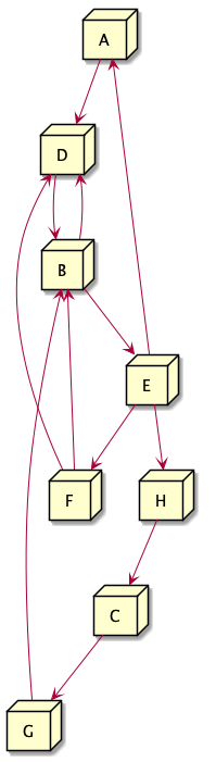
means using an example. Consider the system represented by the directed
graph in Figure 1. This system has eight components represented with the
labels A through H. Arrows represent the directed interactions between
system components. In our example, A makes a directed call to D and
E makes a directed call to F.
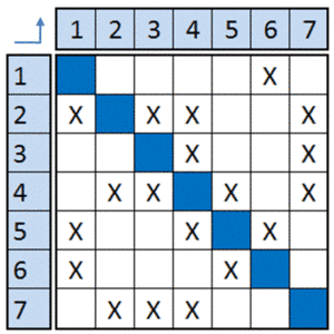
We can represent this same directed graph as a matrix, called a design
structure matrix, or DSM, as in the table below. The cells along the
diagonal of the matrix are the system components A through H. Each X
in the matrix represents an interaction in the system between two
components. You can think of each diagonal cell in the matrix as having
inputs entering from its left and right sides, and outputs exiting from
above and below. For example, reading across row D, we see that
component D has inputs from elements A, B, and F, represented by
the X marks in row D. Reading down column D, we see that D has an
output going to component B. Each X mark in the matrix represents an
interaction between two components that may either be an input or an
output, depending on the perspective you view the matrix from.
| A | B | C | D | E | F | G | H | |
|---|---|---|---|---|---|---|---|---|
| A | A | X | ||||||
| B | B | X | X | X | ||||
| C | C | |||||||
| D | X | X | D | X | ||||
| E | X | E | ||||||
| F | X | F | ||||||
| G | X | G | ||||||
| H | X | H |
By representing our directed graph as a matrix, we already gain a few benefits: the graphical nature of the matrix is highly compact, easily scalable to very large systems, and intuitively readable for representing the connections between components in a system. The matrix representation also unlocks a key capability we didn’t have in the visual representation — mathematical analysis. The matrix-based nature of the DSM opens the door to applying a number of powerful analyses from graph theory and matrix mathematics that allow us to discover important system patterns and effects.
Analyzing an Architecture using a DSM
Let’s turn our effort towards leveraging a DSM to analyze and improve software architecture.
Basic Metrics
The first step in performing this analysis is to look at some of the simple metrics and discover what they mean for our architecture. These metrics are typically graph theoretic and any nodes in the graph having high values may be in some sense more ‘important’, ‘central’ or ‘critical’ to the system.
These metrics were generated using Cambridge Advanced Modeler.
Clustering coefficient
In graph theory, a clustering coefficient is a measure of the degree to which nodes in a graph tend to cluster together. A high clustering coefficient is indicative of a small-world network where the neighbours of any node are likely to also be neighbours of each other. In our service oriented architecture, a high clustering coefficient represents components of subsystems that are highly connected to that subsystem, but little connected to other subsystems.
| Element name | Clustering coefficient |
|---|---|
| F | 0.5 |
| B | 0.166666667 |
| D | 0.166666667 |
| E | 0.083333333 |
| A | 0 |
| C | 0 |
| G | 0 |
| H | 0 |
Betweenness centrality
Betweenness centrality represents the degree to which nodes stand between each other. For example, in a network, a node with higher betweenness centrality would have more control over the network, because more information needs to pass through that node to reach other areas of the network. In a microservice architecture, services with high betweenness centrality may have considerable influence within the system by virtue of their control over information passing through the system. They are also the services whose removal from the network will most disrupt communications between other services because they lie on the largest number of paths between services. These services are typically correlated with critical data paths or single points of failure.
| Element name | Betweenness centrality |
|---|---|
| B | 20 |
| E | 16 |
| G | 6 |
| D | 4 |
| F | 1.5 |
| A | 0.5 |
| C | 0 |
| H | 0 |
In-degree
In-degree is a fairly simple metric tracking the number of edges directed into a vertex in a directed graph. Services with a high in-degree are ones that a lot of teams are making calls too.
| Element name | In-degree |
|---|---|
| B | 3 |
| D | 3 |
| E | 1 |
| G | 1 |
| F | 1 |
| A | 1 |
| H | 1 |
| C | 0 |
Out-degree
Out-degree is the opposite of in-degree — the number of edges directed out of a vertex in a directed graph. Services with a high out-degree are those that make a lot of calls to other services. These services have the highest number of external dependencies and will likely need to take extra care to protect themselves from downstream failures.
| Element name | Out-degree |
|---|---|
| E | 3 |
| B | 2 |
| F | 2 |
| D | 1 |
| G | 1 |
| A | 1 |
| C | 1 |
| H | 0 |
Reachability
Reachability refers to the ability to get from one vertex to another within a graph. Typically, connecting “glue” services like messaging middleware will have high reachability. For example, at Workiva, our linking system used to ensure cross-document consistency has a high reachability.
| Element name | Reachability |
|---|---|
| C | 7 |
| E | 6 |
| B | 6 |
| F | 6 |
| G | 6 |
| A | 6 |
| D | 1 |
| H | 0 |
Clustering Components
Each of the components in our matrix may be a microservice, or it may be a code module developed by a team. One of the basic assumptions we try to make when designing components and software teams is minimizing the coordination overhead between groups to improve overall efficiency of the group (the so-called Inverse Conway’s maneuver). A DSM can help us design an optimal organization by finding the subsets of the matrix that are mutually exclusive or minimally interacting. These “clusters” are groups of elements that are interconnected among themselves while being little connected to the rest of the system.
In other words, clusters absorb most, if not all, of the interactions (i.e. DSM marks) internally and the interactions or links between separate clusters are eliminated or at least minimized.
As a simple example, consider a system that includes seven services and the interactions between those services as shown in the DSM below (example adapted from DSM Web). If we were to form several software development teams to deliver this, how many teams should we have and what services should they be responsible for?
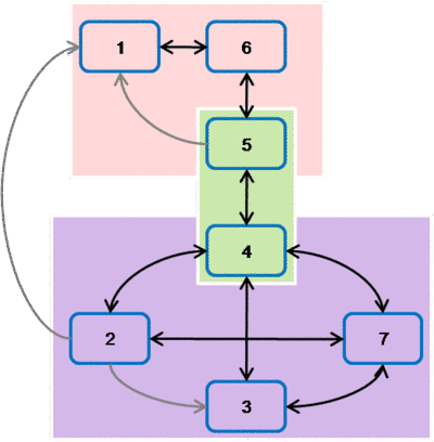
Clustering the DSM for this system will provide us with insights into optimal team formations based on the degree of interactions among services. If the above DSM was rearranged and systems grouped by responsible team, we could come up with the following arrangement.
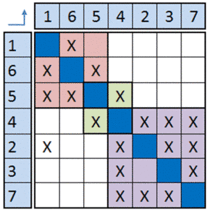
| Team | Services |
|---|---|
| Team 1 | services 1, 5 and 6 |
| Team 2 | services 4 and 5 |
| Team 3 | services 2, 3, 4 and 7 |
Services 4 and 5 provide an interesting insight — each of these services belongs to two logical subsystems. These services will naturally have a higher coordination overhead and will likely require the involvement of an Architect and the support of Delivery Management and Engineering Management to execute on effectively. Drawing out these services clustered by the team assignments highlights the criticality of services 4 and 5 to the success of the overall system.
Clustering a DSM can be viewed as an optimization problem, and there are several iterative algorithms that can be applied to a matrix to find an optimum set of clusters, the original version being developed by Carlos Fernandez and further improved by Ronnie Thebeau as part of a Master’s thesis. This algorithm frames the problem by attaching a cost to interactions between matrix elements, randomly choosing clusterings, and choosing the best fit using a hill-climbing algorithm that settles on an optimum arrangement of clusters. Roughly speaking, the algorithm consists of several steps:
- Place each element in its own initial cluster.
- Calculate the Coordination Cost metric of the current matrix.
- Randomly choose an element.
- Calculate the cost of adding the element to any existing cluster.
- If the new coordination cost is lower than the current coordination cost, make the change of cluster permanent.
- Repeat from step 2 until the algorithm stops making changes.
Cambridge Advanced Modeler provides an implementation of this clustering algorithm that we can use to find the optimal arrangement of services into highly connected groups. In some cases, these groups suggest new ways to divide services between software delivery teams, in others, they suggest areas where Scrum Masters or Software Architects should be involved more deliberately to make sure integration between components is as smooth as possible.
Optimizing Processes
Many software systems are used to model business processes. A simple way to reduce the complexity of the software system is to reduce the complexity of the process it is trying to model. You can think about a process DSM as mapping the flow of code execution. In many processes, the possibility of doing rework due to a failed step contributes to a lot of overhead in the system. These feedback loops, or cycles, can be identified within a DSM through an iterative process called sequencing.
Sequencing re-orders the rows of a DSM to minimize the number of cycles. Intuitively, if we minimize the number of cycles in a process, we also minimize the number of dependencies between steps, resulting in a more efficient overall process. The first heuristic for obtaining a good sequence is to find an ordering that minimizes feedback loops. A secondary heuristic is to minimize the distance between feedback loops where they can’t be avoided. Long feedback loops are problematic because many more steps of the process will have been started by the time we realize that a failure occurred and we will need to restart. There are several iterative algorithms for sequencing a DSM available at DSM Web.
The simplest algorithm to show the concept of process optimization is Steward’s path searching algorithm, outlined as follows:
- Activities with empty rows have no inputs and can be done first, order these at the top of the DSM.
- Activities with empty columns have no outputs and therefore provide no information to any downstream activities, these activities can be done last and should be placed at the end of the DSM.
- Find any cycles in the remaining elements through a depth-first search.
- Group together all activities in a cycle as a single activity, and treat the group as its own step in the sequence.
After this algorithm converges to a steady state, the resulting process will have the fewest number of feedback loops and the steps in the process will be “close”, meaning that each step does not have to spend a long time waiting for inputs.
Next Steps and Future Work
I find the idea of using a structured technique to optimize software architecture compelling, and the next step in leveraging DSM analysis is to apply it to a real-world software project. Tools like Ndepend or Lattix include DSM tools for analyzing the architecture of a single software project. My interest is using these techniques to model a micro-service architecture across an entire organization. By tracking network calls between microservices, we can build up a picture of the dependencies between services and then analyze the resulting system using the techniques presented here, developing new insights into team formation, critical services, and optimum workflows.
Additional Resources
- The Cambridge Advanced Modeler is a software suite with DSM analysis tools.
- An introduction to DSM tools and techniques is available at DSM Web.
- The book Design Structure Matrix Methods and Applications, part of the Engineering Systems series, provides a more thorough introduction to DSM.