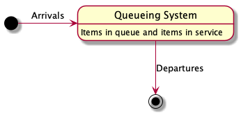
A queueing system can be described as the flow of items through a queue. In a queueing system, items arrive at some rate to the system and join one or more queues inside the system. These items receive some kind of service, and when the work is done, they depart the system.
Little’s Law is a pretty simple model of queueing systems.
$$ L=\lambda W $$
Little’s Law says that the average number of items in a queueing system, denoted \(L\), equals the average arrival rate of items in the system, \(\lambda\), multiplied by the average waiting time of an item in the system, \(W\).
Little’s Law is a useful tool for software architecture because it provides a simple way to measure the effect of changes to a system. For example, as long as we know two of the three numbers, we can always derive the third, and by varying these numbers we can estimate the effect of a change on system performance.
Using Little’s Law to Measure Response Time
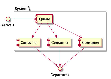
Let’s see how Little’s Law can be used in a practical example. Consider a Competing Consumer system with one queue and three workers.
We can use Little’s Law to calculate response times for each task by moving some of the variables around:
$$ L = \lambda W \rightarrow W = \frac{L}{\lambda} $$
where,
$$ \begin{aligned} W & = \text{response time} \cr L & = \text{work in progress} \cr \lambda & = \text{throughput} \cr \end{aligned} $$
We can use this formulation and some measurements to calculate the response time of the system. Suppose we’ve been running this system for a while and have observed an average queue depth of ten tasks. This number represents the number of tasks in the system and provides \(L\), the work in progress. We also measure the throughput of the system by tracking the number of tasks that each consumer can process per second. In our measurements we’ve observed that each consumer can process on average 10 tasks per second, giving us mean throughput, \(\lambda\). We can use these numbers to derive how long it takes the average task takes to move through the system, \(W\).
$$ \begin{aligned} \text{response time} & = \frac{\text{work in progress}}{\text{throughput}} \cr \text{W} & = \frac{L}{\lambda} \cr \text{response time} & = \frac{10}{30} \text{ seconds} \cr \text{response time} & = \frac{1}{3} \text{ seconds} \cr \end{aligned} $$
By adjusting these numbers, you can simulate the effect of varying the system architecture. For example, suppose we expect the average number of tasks arriving in the queue to increase from 10 to 50 due to an upcoming Black Friday sale. What effect would this have on response time? We can use Little’s Law to find out:
$$ \begin{aligned} \text{response time} & = \frac{\text{work in progress}}{\text{throughput}} \cr \text{W} & = \frac{L}{\lambda} \cr \text{response time} & = \frac{50}{30} \text{ seconds} \cr \text{response time} & = 1 \frac{2}{3} \text{ seconds} \cr \end{aligned} $$
The increased demand on the system increased response time from \(\frac{1}{3}\) of a second to \(1 \frac{2}{3}\) seconds. We’ve been striving to keep response times below a half of a second, so we need to do some work to prepare for this influx of users. How about adding more queue consumers? In our previous measurements we found that each consumers can process about 10 tasks per second. What effect would adding two more consumers to our system have? This brings the total number of consumers to five and the expected mean throughput up from 30 to 50.
$$ \begin{aligned} \text{response time} & = \frac{\text{work in progress}}{\text{throughput}} \cr \text{W} & = \frac{L}{\lambda} \cr \text{response time} & = \frac{50}{50} \text{ seconds} \cr \text{response time} & = 1 \text{ second} \cr \end{aligned} $$
Response time dropped from \(1 \frac{2}{3}\) seconds to one second — not enough change. Let’s take a different approach. Suppose we want to keep our response time at \(\frac{1}{3}\) of a second. How many consumers do we need, assuming each is able to process ten tasks per second? In this problem, we hold \(W\) at \(\frac{1}{3}\), and \(L\) at 50, calculating \(\lambda\).
$$ \begin{aligned} \text{response time} & = \frac{\text{work in progress}}{\text{throughput}} \cr \text{W} & = \frac{L}{\lambda} \cr \frac{1}{3} & = \frac{50}{\lambda} \cr \lambda & = 150 \cr \end{aligned} $$
To keep our response time at \(\frac{1}{3}\) of a second given our increase load, we need to be able to process 150 tasks per second, which would require having 15 consumers able to process 10 requests per second.
Why is Little’s Law Useful in Practice
\(L\), \(\lambda\), and \(W\) are three quite different and important measures of effectiveness of system performance, and Little’s Law insists that they must obey the “law”.
You may have a strong desire to increase system performance by seeking higher throughput (\(\lambda\)), or you may want to lower the length of time a task is waiting in the queue (\(W\)), or you may want to reduce the average number of tasks in the system at a time (\(L\)). Any of these things is achievable, but Little’s Law highlights the interdependencies between these variables, allowing you to understand the implications in making system changes that try and achieve your goals. We can use this simple law to make better decisions.
Remarkably, Little’s Law holds for queueing systems “with any distribution of processing times, ordering, or practically anything else”. Simple ideas can be extremely powerful. Little’s Law is one such idea.