Vector clocks are an extension of Lamport Clocks designed to determine all correct orderings of events in a distributed system. Whereas Lamport Clocks yield one of the many possible event orderings, this does not for certain classes of problems that require knowledge of global program state such as reversing the order of execution to recover from errors or rollback. In such cases, it is more useful to have access to the entire set of orderings that are causally consistent at any moment in time. Vector clocks are designed for exactly such cases.
Vector clocks are first described in 1986 by Rivka Ladin and Barbara Liskov in a paper about distributed garbage collection. Independently, a paper written in 1988 by Colin Fidge uses the term vector clocks to describe the same algorithm, and provides a more complete treatment of the subject which serves as a better introduction to the subject.
Total ordering with Lamport Clocks
Lamport Clocks define a single total ordering of events by having each process maintain an integer value, initially zero, which it increments after every atomic event. These local logical clocks that are incremented per process are synchronized with one another by sending the current local logical clock value on every outgoing message. When a peer in the system receives such a message, it sets its own local logical clock to be greater than this value, if it is not already.
This simple algorithm maintains consistency among the peers since the sending of a message is always set to “happen before” the receipt of the message.
In the following figure, reproduced from the paper, we can see two cases: a) the sending clock is running fast and the clock in the receiver is advanced so that for both systems sending the message happens before its arrival, and b) the sending clock is running slow and now action is required.

Multiple possible orderings
The great thing about Lamport Clocks is that they always report a consistent ordering of events. The less great thing is that they represent only one possible ordering and knowledge of any other ordering is lost. For problems that require knowledge of the global program state, the approach of retaining all possible orders is handled with vector clocks. The aim of vector clocks is to implement the relation \( \rightarrow \) (“happened before”) where \( a \rightarrow b \) if and only if \( a \) must occur before \( b \) in all possible interleaving of events. If \(a \nrightarrow b \) and \( b \nrightarrow a \) then the two events may have occurred concurrently which is denoted \( a \leftrightarrow b \).
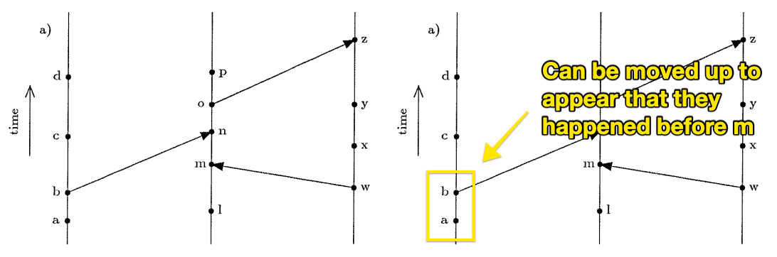
The key to understanding the algorithm is that events between systems form logical “boundaries” that limit the possible number of ways to interleave concurrent events. For example, the following figure shows a single partial ordering of events that is consistent with the Lamport Clock algorithm on the left. On the right, we can note that it is possible to push both \( b \) and \( a \) up in the timeline so that from a global perspective they happen before \( m \). From a causality perspective, both orderings are correct, and from the perspective of an algorithm that cares about global state we may want to know both of these orderings.
The Vector Clock algorithm
To generalize the Lamport Clock algorithm to handle all possible orderings, vector clocks represent timestamps as an array with an integer clock value for every process in the network:
$$ \lbrack c_1, c_2, \mathellipsis c_n \rbrack $$
That is, each process in the network tracks their own logical time as well as the logical time of all other processes in the network.
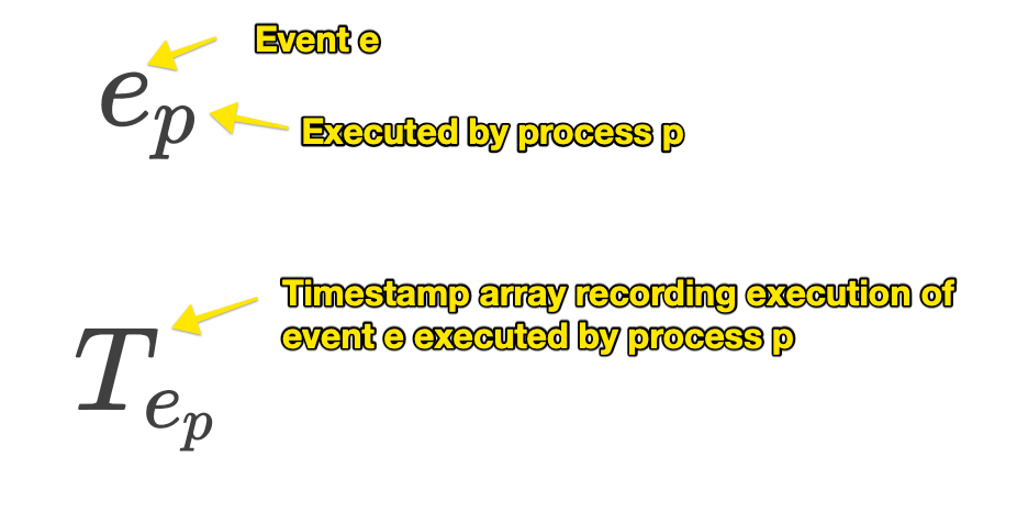
Let \( e_p \) represent an event \( e \) executed by process \( p \), and \( T_{e_p} \) the timestamp array recording the permanent recod of this event execution.
As an example, we can consider the timestamp
$$ [4, 7, 6, 12] $$
that is attached to an event \( x \) that occurs in process \( 2 \). Process \( 2 \) records a local clock value of
$$ T_{x_2}[2] = 7 $$
when this event was executed, and the last known clock value for process \( 4 \) was
$$ T_{x_2}[4] = 12 $$
Note this timestamp is recorded from the perspective of process \( 2 \) and that the local clock in process \(4 \) may have advanced farther but process \(2 \) has only received data up to time \( 12 \).
To maintain the timestamp vector, the following algorithm is used:
- Initially all clocks are zero.
- The local clock value for a process is incremented at least once before each local atomic event (like a database write, or sending a message).
- Each time a process sends a message, it includes a copy of its own timestamp vector.
- Each time a process receives a message, it increments its own logical clock in the vector by one and updates each element in its vector by taking the maximum of the value in its own vector clock and the value in the vector in the received message (for every element).
The following figure from the paper Timestamps in Message-Passing Systems That Preserve the Partial Ordering
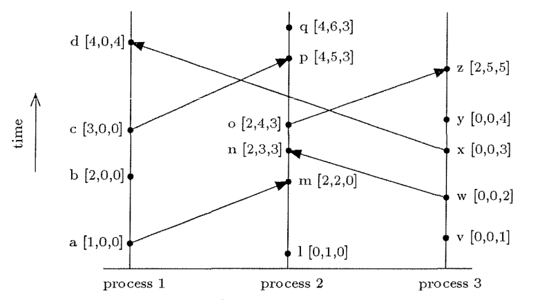
We can note the following “happens before” relationships from the figure:
- For events in the same process
- In process \(3\), \(w \rightarrow y \) since \(2 < 4 \)
- In process \(2\), \(l \rightarrow p \) since \(1 < 5 \)
- In process \(1\), \(c \nrightarrow b \) since \(3 \nless 2 \)
- For the exact same event
- In process \(1\), \(c \nrightarrow c \) since \(3 \nless 3 \), which implies that \(c \leftrightarrow c \)
- In process \(3\), \(y \nrightarrow y \) since \(4 \nless 4 \), which implies that \(y \leftrightarrow y \)
- For events with no causal relationship that happen in different
processes, we compare using the local clock for each process
- \( l \leftrightarrow v\) since \((1 \nless 0) \land (1 \nless 0)\)
- \( d \leftrightarrow z\) since \((4 \nless 2) \land (5 \nless 4)\)
- \( l \leftrightarrow b\) since \((2 \nless 0) \land (1 \nless 0)\)
- For events separated by intervening communication between processes
- \( b \rightarrow q\) since \(2 < 4 \)
- \( w \rightarrow n\) since \(2 < 3 \)
- \( q \nrightarrow c\) since \(6 \nless 0 \)
- \( a \rightarrow z\) since \(1 < 2 \)
Summary
The vector clock algorithm defines the order between two events whenever inter-process communication creates a causal link between the two events. By tracking the logical clock of each process in the system, we make it possible compare and form a globally consistent snapshot of system state. This is useful for applications that require knowledge of global state like garbage collection, or rolling back errors by reversing the order of execution. To learn more about vector clocks, consult the following resources: